Continuing from last time, I would like to talk about digital signal processing (DSP) in radiation measurement, comparing it with analog Gaussian shaping.

This time, I would like to focus on high count rates.

When utilizing a coaxial HPGe detector for gamma-ray spectroscopy, optimal resolution is typically achieved using Gaussian shaping with a 6 μs time constant. As the counting rate increases, however, the dead time also increases.

For instance, at an input counting rate of 6,000 cps, the dead time can exceed 20%. In such scenarios, resolution may need to be compromised, and the time constant may be reduced to accommodate higher count rates.

Analog Gaussian shaping, although effective, can face limitations due to ballistic deficit that may necessitate shortening the shaping time to 2 μs. Reducing it further to 1 μs can lead to noticeable ballistic effects, resulting in spectral asymmetry and degraded resolution. For higher count rates, gated integrator shaping proves beneficial in analog setups, a topic which could be explored in a separate article.

Fig. 1 Comparison of DSP and AMP pulse response

Let's compare trapezoidal shaping and Gaussian shaping.

In Fig. 1, the blue trace represents the signal from the preamplifier, the green trace corresponds to the amplifier time constant of 2μs for the preamplifier, and the purple trace shows the waveform with a DSP risetime of 4.4μs.

Trapezoidal shaping returns to the baseline faster than Gaussian shaping. This means that preparations for accurately measuring the next pulse can be made faster with trapezoidal shaping, and the output count rate is higher with trapezoidal shaping.

Fig. 2 Comparison of output count rate of DSP and AMP

As can be seen from Fig. 2, both the amplifier and DSP are almost linear up to an input count rate of 5kcps. The amplifier starts to deviate from the straight line at about 6kcps. I estimate the DSP is around 20kcps. The amplifier also adds the MCA conversion time (1μs) as dead time, so it doesn't take as long as you might think.

Fig. 3 Change in resolution

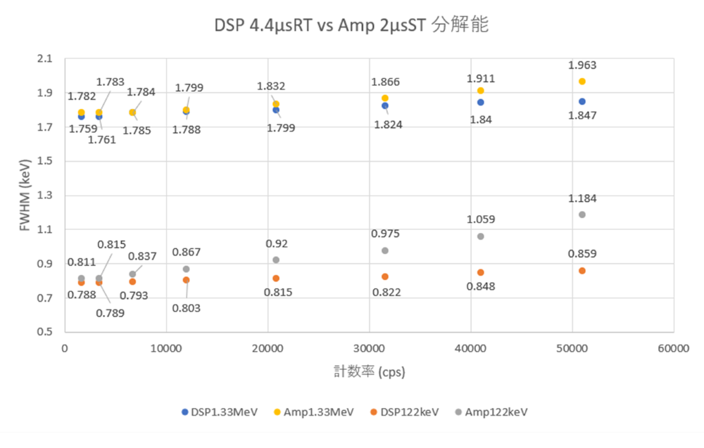
The resolution is about the same up to about 12kcps. Beyond that, the difference gradually widens. This is especially noticeable at low energies of 122keV.

From Fig. 3, it can be seen that DSP has a shorter time constant (rise time) and can demonstrate its true value especially at high counting rates. I believe this is also possible because of the robust BLR (Base Line Restorer) algorithm.

Now, all of our employees will do their best to create even better products. Thank you very much for your support.