In this section, we will discuss the peak area calculation for peak search analysis, a spectrum analysis function available in our DSP and MCA systems.

Techno AP’s peak search analysis employs the Cobel method for peak area calculation.

Unlike the basic total peak area method, which integrates counts within regions of interest (ROIs) in gamma-ray spectra and provides a raw gross count, the Cobel method accounts for background interference.

The total peak area approach does not factor in background counts, which can lead to inaccuracies due to the baseline often containing continuous spectra from Compton-scattered gamma rays and natural radiation.

This background can cause a downward slope in the peak’s baseline. The Cobel method is preferred for its simplicity and reliability in such cases.

The values net (count)raw and net (cps)raw are derived by applying the Cobel method to the raw data of yi. Conversely, net (count)fit and net (cps)fit are calculated using the Cobel method on data adjusted through Gaussian fitting f (xi;a).

The Cobel method estimates the baseline area by analyzing the channels at both ends of the peak region (see Fig. 1).

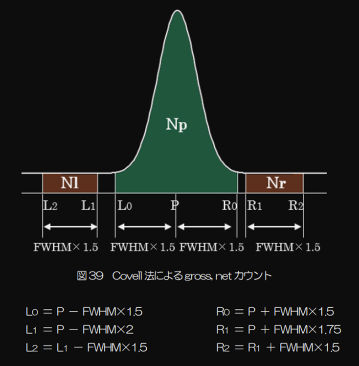
Fig.1 Conceptual diagram of the Cobel method

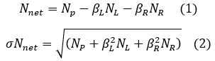
The peak area (Nnet) and its standard deviation (σNnet) are expressed by the following formula:

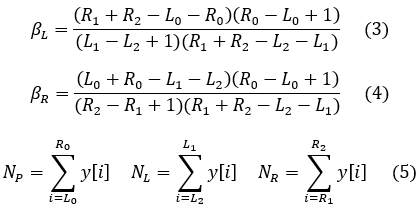
　βL,βR are the counts used to convert NL NR to baseline counts.

This calculation can be implemented efficiently using a simple for loop in C and optimized further by compiling it into a DLL (Fig. 2).

This approach will enable us to compute the net counts, net(count)raw and net(count)fit, more quickly.

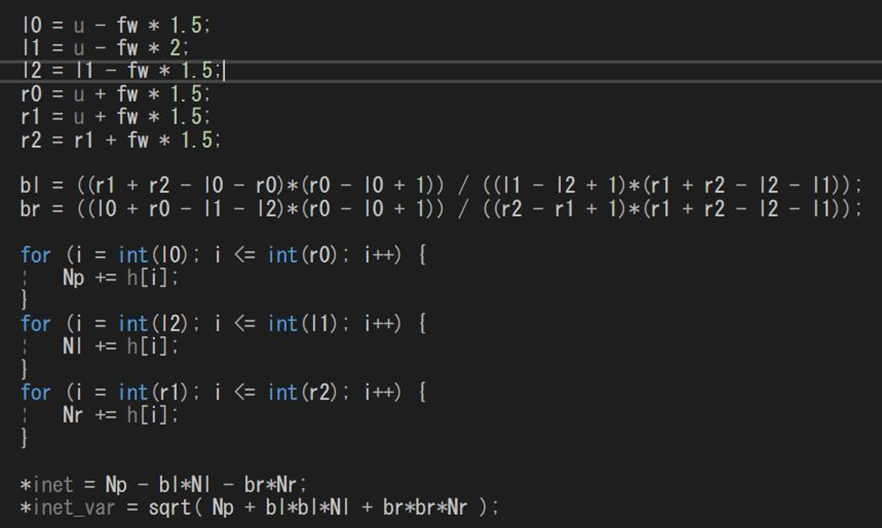
Fig.2 Cobel method code

In measurement systems, there is a minimum time interval required for two events to be recorded as separate pulses by the detector signal.

This interval, known as the dead time, can be influenced by both the internal processes of the detector and the associated electronic circuitry. Due to the random nature of radioactive decay, if an event occurs too soon after the previous one, it cannot be recorded and will be lost.

As the count rate increases, the dead time becomes more significant, leading to greater data loss. Therefore, a system that compensates for dead time (dead time correction) becomes increasingly necessary. The dead time correction is handled by the MCA (DSP), which includes the following components:

MCA dead time = Linear gate time TLG + (ADC conversion time + memory recording time)TM (6)

The linear gate time TLG is the duration required for the signal from the detector to be processed by the AMP (DSP) and reach its peak. This time is necessary to measure the pulse height (energy) and constitutes the dead time. As illustrated in Fig. 3, this is estimated to be around 14 μs.

The ADC conversion time follows. In DSP systems, this time is relatively short due to the pipeline sampling of the preamp waveform, typically ranging from 10 ns to 40 ns.

In contrast, MCAs use successive approximation ADCs with conversion times ranging from 500 ns to 5 μs, including the time required to reset the peak-held charge. Modern MCAs may use digital sampling techniques, where a pipeline ADC detects the peak top of the amplifier signal digitally, allowing conversion times to be reduced to 10 ns to 40 ns.

Currently, the time required to record memory is typically just a few tens of nanoseconds due to its storage in the FPGA, making it nearly negligible.

The ADC conversion time combined with the memory recording time can be considered the MCA processing time, TM.

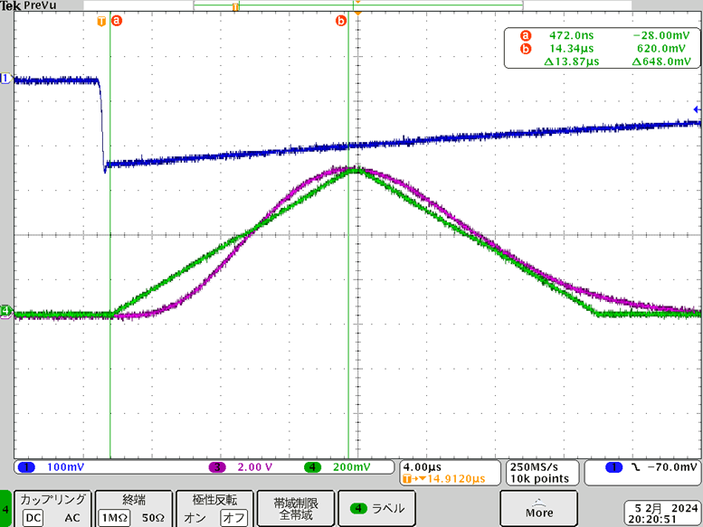
Fig.3 DSP and AMP Pulse Response to Preamp Signal input

The probability of dead time occurring is the chance that the next pulse won't arrive during the pulse processing time (TLG + TM). If a pulse arrives during this period, it will either be removed or gated out.

Next, consider the probability that a pulse will not arrive during the linear gate time TLG.

When pile-up is active, if multiple pulses arrive during TLG, all pulses will be removed. If additional pulses arrive during TM, the preceding pulses are processed while the subsequent ones are gated out.

In other words:

PP = TLG + Probability of no pulse during TM × Probability of no pulse during TLG (7)

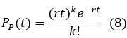
The random events of radioactive decay can be predicted by the Poisson distribution, which gives the probability of obtaining k counts within time t, assuming an average count rate of r [cps], as follows:

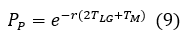
By substituting k=0 (no pulse arrives), t=TLG+ TM into equation (7) and t= TLG into equation (8), and then multiplying the results, we obtain the following equation:

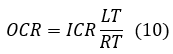
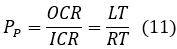
The processed pulse probability PP can also be expressed as the ratio of the OCR (output count rate) to the ICR (input count rate). Additionally, OCR can be viewed as a product of ICR and the Livetime/Realtime ratio from a different perspective.

In other words,

LT(LiveTime)is

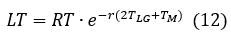
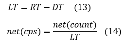
LT (LiveTime) performs dead time correction from Eq (12). Livetime becomes Eq(13).

Figures 5, 6, and 7 show spectra used to assess the effectiveness of dead-time correction with a Cs-137 single peak source.

Focus on the net counts in these spectra. If dead-time correction is not applied, equation (14) will use Realtime rather than Livetime.

As showen in Fig. 5, at high counting rates, net counts (cps) are noticeably lower when measured with a longer rise time.

Fig.4 Comparison of net(count)/RT at each risetime

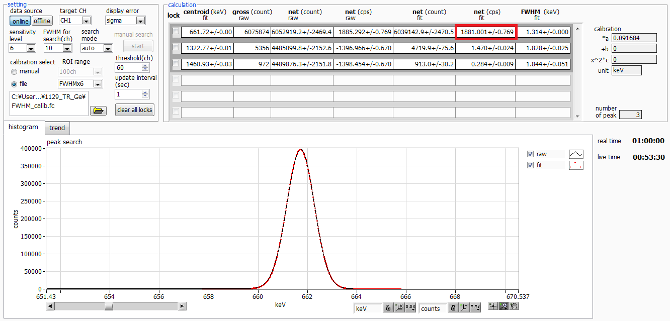
Fig. 5 Cs-137 spectrum with HPGe, ICR 11 kcps, risetime 4000 ns, flattop 800 ns.

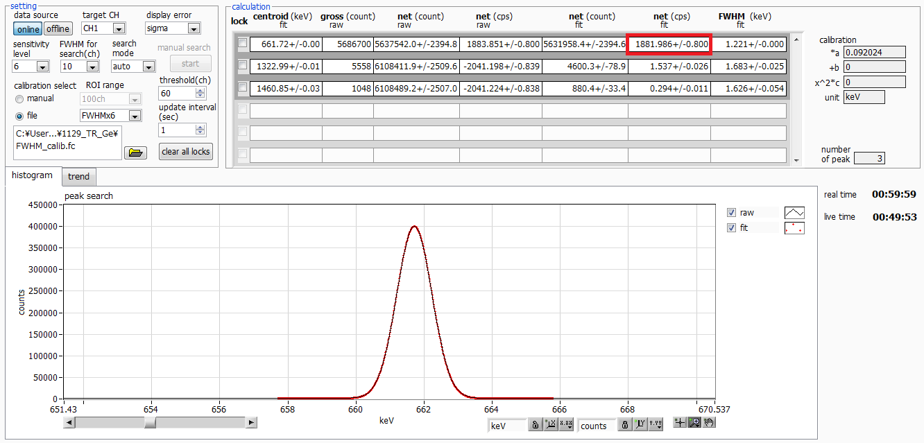
Fig. 6 Cs-137 spectrum with HPGe, ICR 11 kcps, risetime 7200 ns, flattop 800 ns.

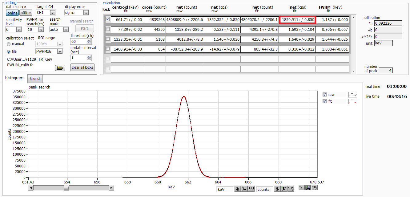
Fig. 7 Cs-137 spectrum with HPGe, ICR 11 kcps, risetime 14000 ns, flattop 800 ns.

Now, focus on the net(cps) values in Figures 5, 6, and 7.

These values are corrected for dead time, meaning they are divided by Livetime (LT).

As shown in Fig. 8, even with a longer rise time at high counting rates, the error is kept within 1.6%, making it practical. The FWHM improves with longer rise times, leading to better resolution, thus demonstrating the effectiveness of dead-time correction.

Fig.8 Cs-137 Spectrum with HPGe, ICR 11kcps, risetime 14000ns, and flattop 800ns.

Our team is dedicated to delivering even better products, and we greatly appreciate your continued support. Thank you.

References
[1] Gordon, Gilmore, Practical Gamma-Ray Spectrometry, John Wiley & Sons Ltd, 1995.
[2] Glenn F. Knoll, Radiation Detection and Measurement, 4th Edition, Ohmsha, 2013.